
Reading a Qubit Before It Changes Its Mind: A Sub-Microsecond LSTM on AI Engines and FPGA Fabric
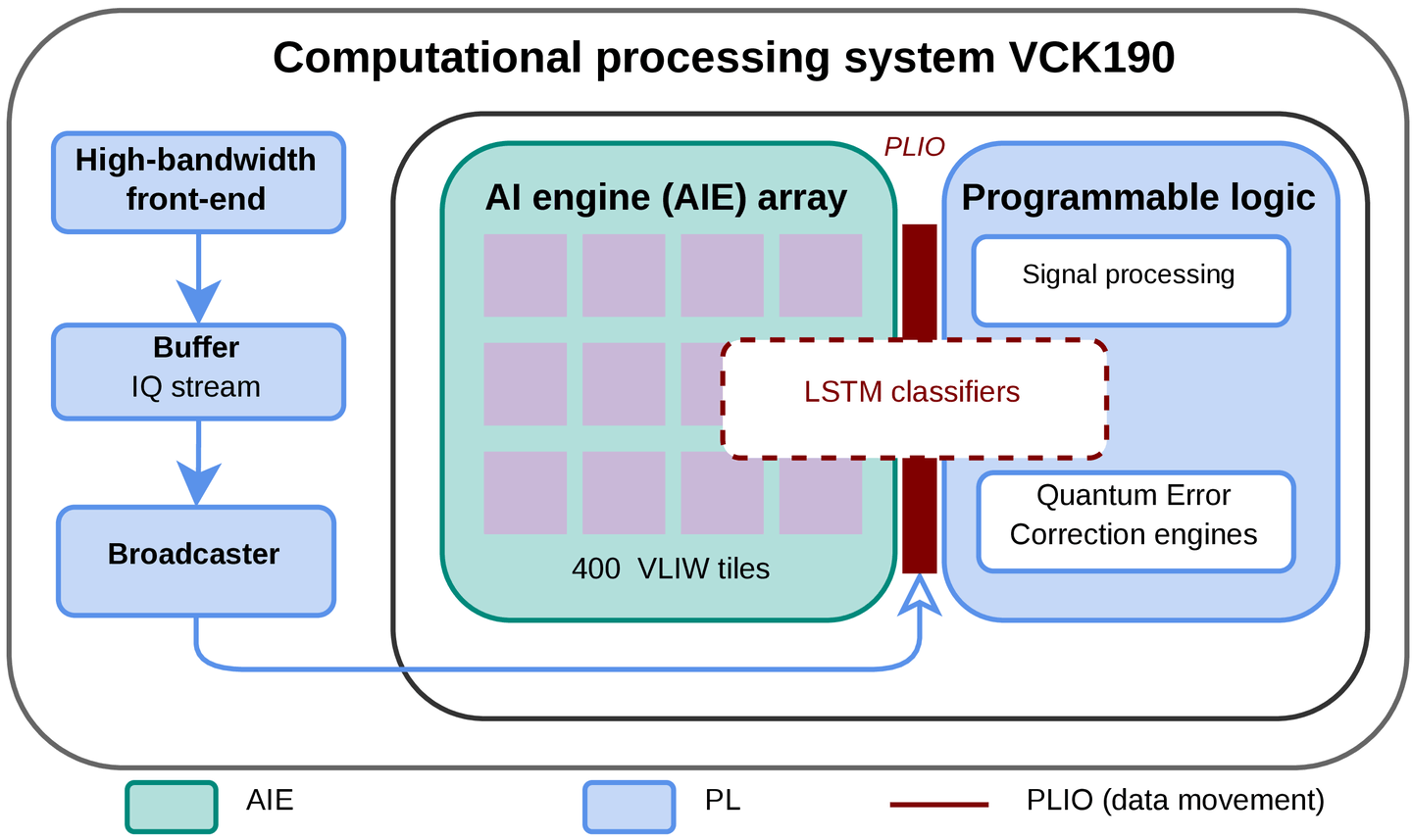
This post walks through our preprint Real-Time Recurrent Qubit-State Discrimination on a Heterogeneous AI-Engine–FPGA Accelerator (v2), joint work with Yilun Xu, Neel Vora, Gang Huang, Deepak Ganesan and Phuc Nguyen (UMass Amherst and Lawrence Berkeley National Laboratory).
TL;DR. Some qubits “change their mind” partway through a measurement. Spotting that needs a model that reads the signal over time, which is usually too slow or too big for a 1 µs deadline. We split a small LSTM along its data dependencies: the parallel part runs on 4 of the 400 AI Engine tiles of an AMD Versal chip, and the step-by-step part runs in the FPGA fabric. On the hardest qubit it matches a far larger network’s accuracy (96.59% vs. 96.37%) with 403× fewer parameters, and answers in 860 ns measured on real hardware.
Asking a qubit “0 or 1?”, fast
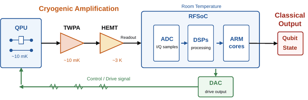
A quantum computer keeps asking its qubits one question: which state are you in? This step is called readout, and in superconducting processors it is one of the slowest and most error-prone operations. It also sits on the critical path. If the controller has to react to the answer, for example to apply a correction, the answer has to come back quickly. In our setup the accelerator has 1,000 ns, starting from the first sample of the readout signal.
Here is what a readout looks like. A microwave pulse bounces off a resonator coupled to the qubit, and the qubit’s state slightly shifts the phase and amplitude of the reflected wave. Electronics digitize it into two streams, I and Q (in-phase and quadrature). With the QubiC control system sampling at 2 GSPS, a 704 ns readout window gives 1,408 complex samples (2,816 numbers) per shot. A classifier must turn those numbers into a label: |0⟩, |1⟩ or |2⟩ (transmon qubits have a third level that we also classify).
When the qubit changes its mind
The standard trick is to integrate: average the whole trace down to a single (I, Q) point, then decide which cluster it falls in. It is cheap, and for most qubits it works very well.
But a qubit in |1⟩ can relax to |0⟩ in the middle of the measurement. Its early samples still say “1”, but its later samples look like “0”. Integration blends the two together, a bit like a long-exposure photo of a moving car, and the point lands in the wrong place.
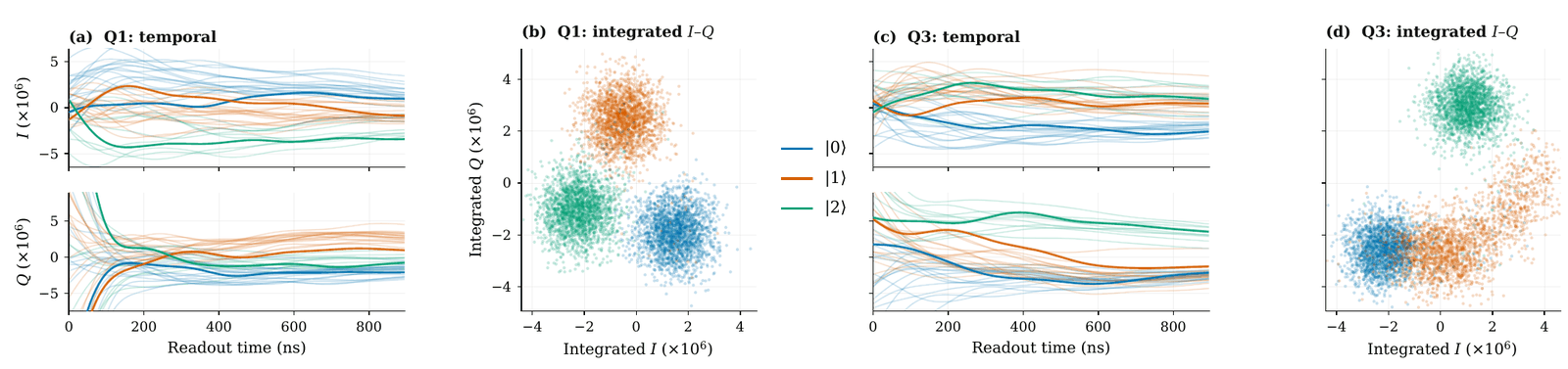
We saw this clearly on one qubit in our dataset, Q3. On Q3 at 704 ns:
- A Gaussian mixture model on the integrated point (GMM) reaches 89.27%.
- A better learned decision boundary on the same point (QubiCML) reaches 93.95%.
- A full-resolution feed-forward network that sees all 2,816 values (FCN) reaches 96.37%.
So better boundaries only get you part of the way. The rest of the accuracy is in the timing of the signal. A longer window even makes integration worse on Q3: GMM drops from 92.53% at 512 ns to 88.99% at 768 ns, because more of the late “0-like” signal gets mixed in.
The catch is that the FCN needs millions of parameters. By our estimates it would use about 89% of the chip’s DSP blocks and take about 9 µs. It recovers the information, but it is not something you can deploy.
Interestingly, only one of our eight qubits behaved like Q3. The other seven do almost as well with integrated inputs. That observation shapes the whole design: the amount of time detail a classifier keeps should be chosen per qubit, not fixed for the whole device.
Enter the LSTM
A recurrent network such as an LSTM is a natural middle ground. It reads the trace one chunk at a time and keeps a small “memory” (the hidden state) of what it has seen so far. Because the memory has a fixed size, the model stays small even when the input is long. It can also start working while samples are still arriving, instead of waiting for the whole trace.
We cut the 704 ns window into 11 steps of 64 ns (128 complex samples each) and use a hidden state of just 8 numbers. We built two variants:
- LSTM-heavy sees all 256 raw values in each step. We use it for difficult qubits like Q3.
- LSTM-compact sees only the average I/Q pair in each step (2 values), so it keeps coarse timing at a tiny cost. We use it for the other qubits.
Compared with the FCN, LSTM-heavy matches Q3 accuracy with 403× fewer parameters. So far, so good. The hard part is the hardware.
Why the obvious hardware mappings fail
Our target is an AMD Versal VCK190. It has two very different kinds of compute on one chip:
- an array of 400 AI Engine (AIE) tiles: small vector processors at 1.25 GHz, very good at wide, parallel multiply-accumulates;
- programmable logic (PL): FPGA fabric at 500 MHz, where you can build custom pipelines and keep data in local registers.
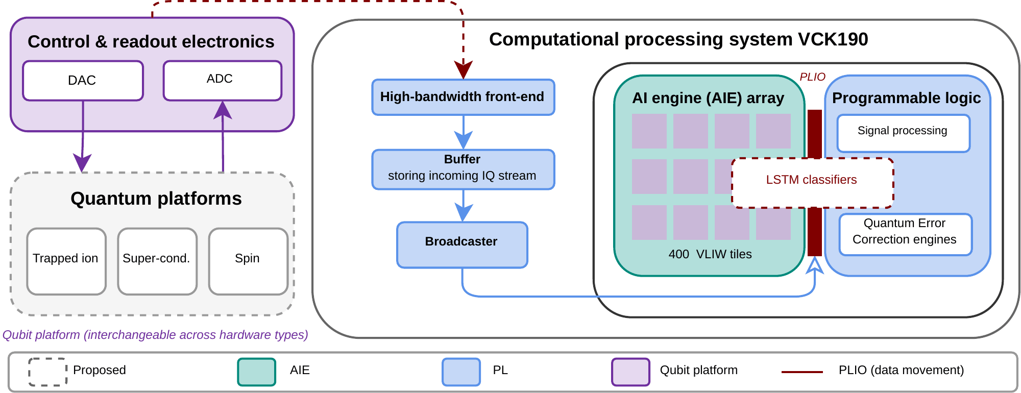
An LSTM step has a nasty property: step t cannot start until step t − 1 has finished, because it needs the previous memory. A new 64 ns chunk arrives every 64 ns, so each update has to finish within 64 ns, every single step.
All on AI Engines? Each AIE tile has only 16 vector registers. The LSTM’s live state needs about 15 of them by our count. The compiler could not fit it and spilled values to memory, which stretched each step to 100 cycles (80 ns at 1.25 GHz). That is longer than the 64 ns budget, so the engine falls behind the input stream. End to end it takes 1,082 ns and misses the deadline. The problem is not a lack of arithmetic. It is register pressure.
All in programmable logic? This keeps pace, but LSTM-heavy then uses 26.9% of the chip’s DSP blocks for a single qubit. A real processor has many qubits to read, so this does not scale.
The idea: cut the LSTM where its dependencies split
Look at what an LSTM computes at each step:
gatest = Wx·xt + Wh·ht−1 + b
The two terms behave very differently:
- Wx·xt (the input projection) depends only on the new chunk, so all four gates can compute it in parallel, as soon as the samples arrive. For LSTM-heavy it is also the big part: 32× more work than the recurrent term.
- Wh·ht−1 (the recurrent projection) is small (8 × 8 per gate), but it depends on the previous step, so it sits on the step-to-step chain.
So we put each part where it fits best. The four input projections go to four AIE tiles, one per gate. The small recurrent update and the final classifier stay in the PL, where the hidden state never leaves local registers.
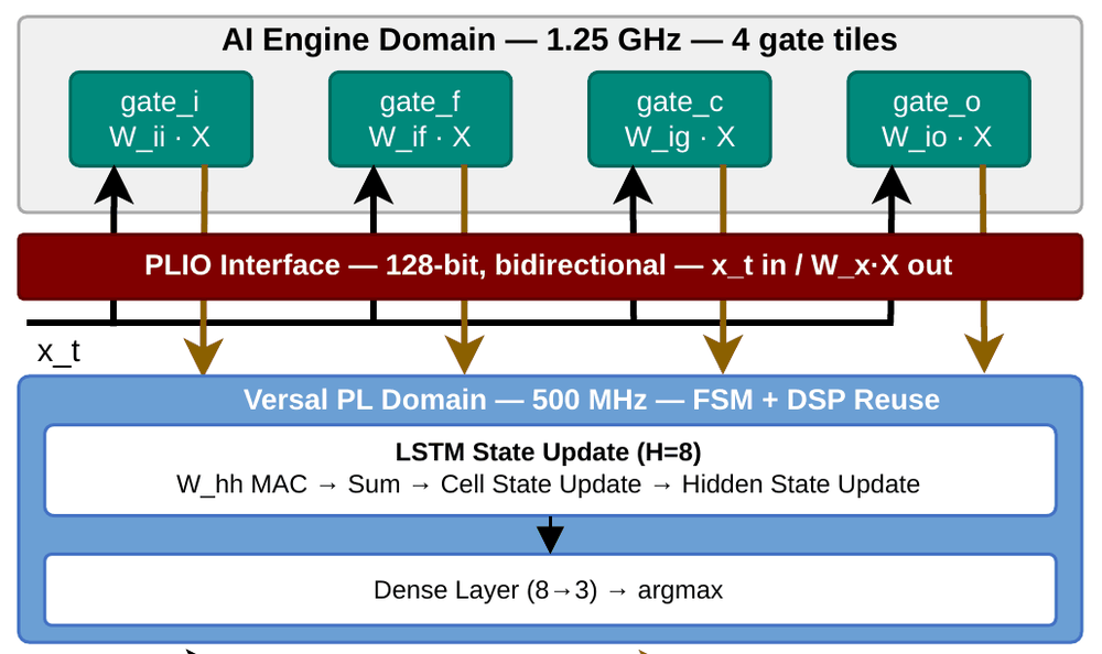
The two halves overlap in time. While the AIE tiles project chunk t, the PL finishes the update for chunk t − 1. The AIE kernel takes 73 cycles (58.4 ns), within the 64 ns budget. The PL update takes 31 cycles (62 ns), and only 18 of those cycles are not hidden behind the AIE work. When the last sample arrives, only a 150 ns tail of work is left, compared with 378 ns for the pure-AIE version.
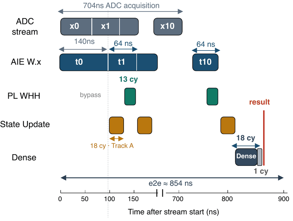
A few details make this work in hardware:
- We swap sigmoid and tanh for hard, clamp-style versions that are cheap in logic. This changes mean accuracy by only a few hundredths of a percentage point (+0.03 for LSTM-heavy, −0.04 for LSTM-compact).
- The deployed datapath uses int16 arithmetic. The mean accuracy loss from quantization is at most 0.05 points.
- Everything is statically scheduled, with no data-dependent control flow, so every shot takes the same time.
Choosing the model with the hardware in mind
We did not pick these sizes by trial and error on accuracy alone. An analytical model of the chip checks three things for each candidate: can the AIE side keep up with the stream, can the PL update keep up, and does the total latency fit in 1,000 ns. Candidates that fail are discarded before training. The search covered hidden sizes 4/8/16, step sizes from 64 to 512 samples, raw vs. averaged inputs, and one or two layers. It turned up a few lessons:
- 64-sample steps are too fast. The PL update cannot finish in time.
- A hidden size of 16 doesn’t help. It doubles the AIE tiles without improving Q3 accuracy.
- A second LSTM layer doesn’t help. It adds hardware and gives no accuracy gain.
One more lesson: the AIE offload is not always worth it. LSTM-compact has only 2 input values per step, so there is too little work to justify the trip to the AIE array. Its PL-only version is faster (814 ns vs. 864 ns), so that is the one we deploy. Where each part runs is a per-model decision, just like how much time detail to keep.
How well does it work?
Accuracy on the hard qubit. On Q3, LSTM-heavy reaches 96.59%, the highest of every classifier we evaluated. Compared with GMM that is 68.2% fewer errors, compared with QubiCML 43.6% fewer, and compared with MF-NN 16.82% fewer. It also edges out the full-resolution FCN (96.37%), although that small gap (6.06% fewer errors) is not statistically significant after correction (p = 0.06). The honest summary is that it matches the FCN with 403× fewer parameters.
Across all eight qubits. LSTM-compact has the highest mean accuracy, 96.78%. Deployed per qubit (LSTM-heavy on Q3, LSTM-compact everywhere else), our design beats the FCN’s readout fidelity on every one of the eight qubits, by 0.07 to 0.54 points (0.29 on average).
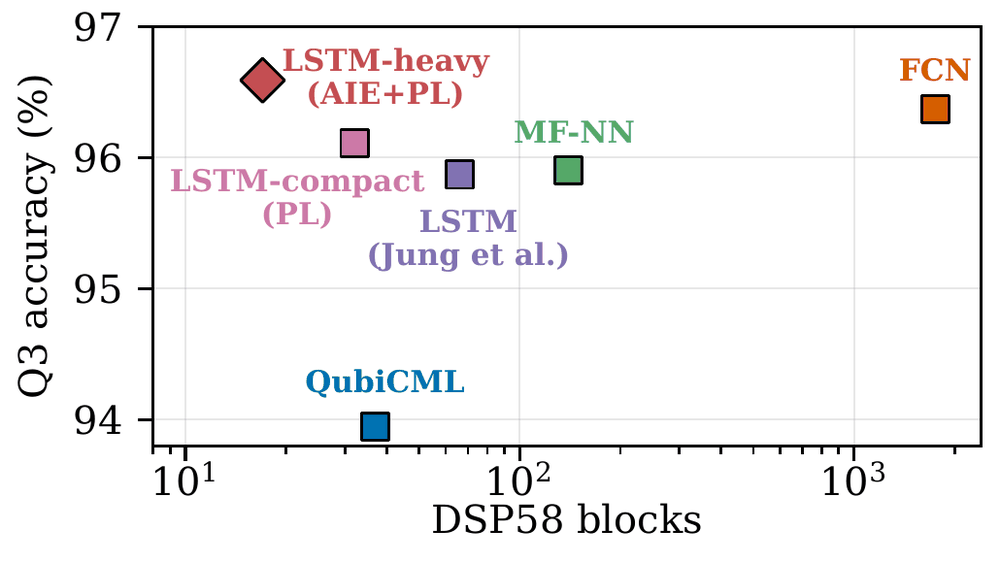
Hardware cost. The DSP blocks are the scarce resource here, and this is where the gap is largest:
| Classifier | Q3 accuracy | DSP58 blocks | Accelerator latency |
|---|---|---|---|
| QubiCML | 93.95% | 37 | 734 ns |
| MF-NN | 95.90% | 140 | 800 ns |
| FCN (estimated) | 96.37% | 1,753 | ~9.19 µs |
| LSTM-compact (PL) | 96.11% | 32 | 814 ns |
| LSTM-heavy (AIE+PL) | 96.59% | 17 + 4 AIE tiles | 854 ns (860 ns measured) |
LSTM-heavy uses 2.2× to 8.2× fewer DSP blocks than QubiCML and MF-NN, and 3.9× fewer than a prior LSTM readout design. Compared with putting the same model entirely in the PL, the hybrid split cuts DSP usage by 31.1× (26.9% → 0.86% of the chip), LUTs by 6.4×, and removes all 128 block RAMs.
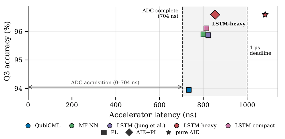
Latency. Both LSTM-heavy versions give the same 96.59% on Q3, since they run identical weights. The difference is the deadline: the AIE+PL split finishes in 854 ns (simulated), while pure AIE takes 1,082 ns. That is a 60.3% shorter tail. We then ran the AIE+PL design on a physical VCK190 board and measured 860 ns end to end, within 0.7% of the simulated figure and inside the 1 µs budget.
What we took away
- Not every qubit needs the same classifier. Time detail matters a lot on some channels and barely at all on others. Choosing per channel saves a large amount of hardware.
- Small recurrent models are limited by registers, not arithmetic. On spatial accelerators like AI Engines, the step-to-step state is what hurts.
- Split the work along its dependencies. Parallel work goes to the AIE array and sequential work to the FPGA fabric. Sometimes the right answer is not to offload at all.
Limitations and what’s next
To be clear about what we did and did not show: apart from the on-board latency measurement, the results come from offline evaluation. We replay recorded readout data into the accelerator at the real 2 GSPS rate; we have not yet run it against live qubits in a fridge. Our latency also covers only the accelerator. It does not include the analog front end, digital down-conversion, the transfer between the QubiC board and the VCK190, or the return path to the controller.
Next, we want to connect the accelerator to a live control loop and scale it to many qubits at once, where AIE tiles and the links between AIE and PL become shared resources. Newer RF-series Versal chips put the data converters on the same chip as the AI Engines and PL, which would remove the board-to-board hop altogether.
Read the paper: arXiv:2610.33843. Questions or comments are very welcome. You can reach me through my website.
(Updated: )